Complex Example
Here we have a more complex example
  1import rf_linkbudget as rf
  2import matplotlib.pyplot as plt
  3import numpy as np
  4import pandas as pd
  5
  6
  7def example():
  8
  9    cr = rf.Circuit('Example')
 10
 11    dup = rf.Attenuator("Duplexer",
 12                        Att=[1.5])
 13
 14    lim = rf.Attenuator("Limiter",
 15                        Att=np.array([0.5, 6.5, 12.5, 18.5]),
 16                        IIP3=60,
 17                        OP1dB=30)
 18
 19    sw1 = rf.SPDT("SW 1",
 20                  Att=0.3)
 21
 22    lna = rf.Amplifier("LNA",
 23                       Gain=[(0, 18.2)],
 24                       NF=0.7,
 25                       OP1dB=21.5,
 26                       OIP3=40)
 27
 28    sw2 = rf.SPDT("SW 2",
 29                  Att=0.3)
 30
 31    att_fix = rf.Attenuator("Att Fix1",
 32                            Att=[1.5])
 33
 34    rxfilt = rf.Attenuator("Rx Filter",
 35                           Att=[2.0])
 36
 37    att_fix2 = rf.Attenuator("Att Fix2",
 38                             Att=[1.5])
 39
 40    driver = rf.Amplifier("Driver",
 41                          Gain=[(0, 14.9)],
 42                          NF=1.7,
 43                          OP1dB=21.4,
 44                          OIP3=40)
 45
 46    dsa = rf.Attenuator("DSA",
 47                        Att=np.arange(1.0, 29, 1.0))
 48
 49    adc = rf.Amplifier("ADC",
 50                       Gain=[(0, 0)],
 51                       OP1dB=-1,
 52                       OIP3=34,
 53                       NF=19)
 54
 55    src = rf.Source("Source")
 56    sink = rf.Sink("Sink")
 57
 58    src['out'] >> dup['in']
 59    dup['out'] >> lim['in']
 60    lim['out'] >> sw1['S']
 61
 62    sw1['S-1'] >> lna['in']
 63    lna['out'] >> sw2['S-1']
 64    sw1['S-2'] >> sw2['S-2']
 65
 66    sw2['S'] >> att_fix['in']
 67    att_fix['out'] >> rxfilt['in']
 68    rxfilt['out'] >> att_fix2['in']
 69    att_fix2['out'] >> driver['in']
 70    driver['out'] >> dsa['in']
 71    dsa['out'] >> adc['in']
 72    adc['out'] >> sink['in']
 73
 74    # create callback function
 75    def cb_src(self, f, p):
 76        return {'f': f, 'p': p, 'Tn': rf.RFMath.T0}
 77
 78    src['out'].regCallback(cb_src)
 79
 80    # create callback function
 81    def cb_lim(self, f, p):
 82        tb = {-31: 6, -30: 6, -29: 6, -28: 6, -27: 6, -26: 6, -25: 12, -24: 12, -23: 12, -22: 12, -21: 12, -20: 12, -19: 18, -18: 18, -17: 18, -16: 18, -15: 18, -14: 18, -13: 18, -12: 18, -11: 18, -10: 18,}
 83        if(p in tb):
 84            self.setAttenuation(tb[p])
 85        else:
 86            self.setAttenuation(0.0)
 87        return {}
 88
 89    lim['in'].regCallback(cb_lim)
 90
 91    # create callback function
 92    def cb_dsa(self, f, p):
 93        tb = {-37: 0, -36: 1, -35: 2, -34: 3, -33: 4, -32: 5, -31: 0, -30: 1, -29: 2, -28: 3, -27: 4, -26: 5, -25: 0, -24: 1, -23: 2, -22: 3, -21: 4, -20: 5, -19: 0, -18: 1, -17: 2, -16: 3, -15: 4, -14: 5, -13: 6, -12: 7, -11: 8, -10: 9,}
 94        if(p in tb):
 95            self.setAttenuation(tb[p])
 96        else:
 97            self.setAttenuation(0)
 98        return {}
 99
100    dsa['in'].regCallback(cb_dsa)
101
102    # create callback function
103    def cb_sw1(self, f, p):
104        if(p > -11):
105            self.setDirection('S-2')
106        else:
107            self.setDirection('S-1')
108        return {}
109
110    sw1['S'].regCallback(cb_sw1)
111    sw2['S'].regCallback(cb_sw1)
112
113    cr.finalise()
114
115    return cr
116
117
118if __name__ == "__main__":
119
120    # define circuit
121    cr1 = example()
122
123    # simualte
124    sim1 = cr1.simulate(network=cr1.net,
125                        start=cr1['Source'],
126                        end=cr1['Sink'],
127                        freq=[0],
128                        power=np.arange(-50, -10, 1.0))
129
130    # key's of interest
131    # only these keys show up in the plots
132    keys1 = [cr1['Source']['out'],
133             cr1['Duplexer']['out'],
134             cr1['Limiter']['out'],
135             cr1['SW 1']['S'],
136             cr1['SW 1']['S-1'],
137             cr1['LNA']['out'],
138             cr1['SW 2']['S'],
139             cr1['Att Fix1']['out'],
140             cr1['Rx Filter']['out'],
141             cr1['Att Fix2']['out'],
142             cr1['Driver']['out'],
143             cr1['DSA']['out'],
144             cr1['ADC']['out'],
145             cr1['Sink']['in']]
146
147    # set noise bandwidth to smallest subband
148    sim1.setNoiseBandwidth(15e3)
149
150    # plot system parameter
151    h = sim1.plot_chain(keys=keys1)
152    k = sim1.plot_total(['NF', 'DYN'])
153    t = sim1.plot_total_simple(['SFDR', 'SNR'], freq=0)
154    k = sim1.plot_total(['NF', 'DYN'])
155
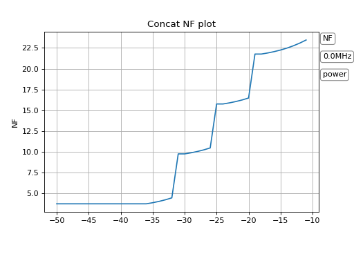
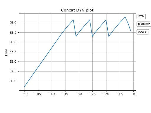
With the plot_total function we can show the NoiseFigure and the Dynamic of the system.
(Source code, png, hires.png, pdf)
(Source code, png, hires.png, pdf)
We see steps in the noisefigure over the input power level. We see that these steps are from the limiter attenuator called lim / Limiter. The limiter is in front of the LNA which is not optimal.
We also see that the overall dynamic has losses exactly at the same input levels. Which is not surprising.
(Source code, png, hires.png, pdf)
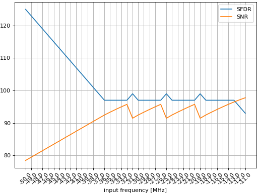
When we compare the SNR and the SFDR view in a plot_total_simple we see something interesting. We see the sweet spot between SNR and the spurious free dynamic range. To have an optimal system means we have to optimize the circuit in a way, so that SFDR and SNR are equal over the hole input power range.
SNR / SFDR optimisation
To optimize the SNR / SFDR we have to keep the signal power of each component in view.
(Source code, png, hires.png, pdf)
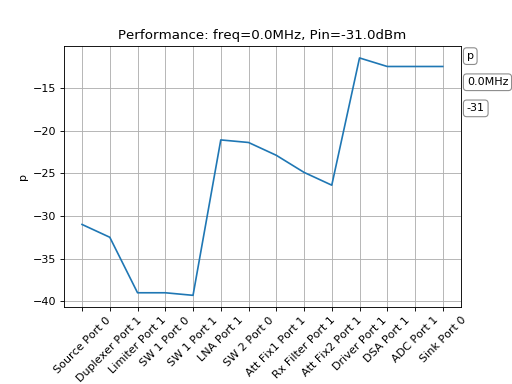
Here in this plot we got an input power of -32dBm. The Driver Amplifier is at an output power of approx -6dBm. And the ADC level is approx at -12dBm which leads to approx -13dBFS. But already with the next higher input power level we have to adjust the ADC input level, otherwise the IM3 components will dominate the hole dynamic. At -31dBm the limiter was activated and will attenuate approx 6.5dB. We see this in the other figures as the krack in the performance. But it is necessary. Otherwise the spurious would dominate and our signal would have an overall worse dynamic.