Analyse and Plotting

We go back to our first example:

import rf_linkbudget as rf
import matplotlib.pyplot as plt
import numpy as np

cr = rf.Circuit('SimpleEx')

lna = rf.Amplifier("LNA TQL9066",
                   Gain=[(0, 18.2)],
                   NF=0.7,
                   OP1dB=21.5,
                   OIP3=40)

drv = rf.Amplifier("Driver TQP3M9028",
                   Gain=[(0, 14.9)],
                   NF=1.7,
                   OP1dB=21.4,
                   OIP3=40)

src = rf.Source("Source")
sink = rf.Sink("Sink")


src['out'] >> lna['in']
lna['out'] >> drv['in']
drv['out'] >> sink['in']


# create callback function
def cb_src(self, f, p):
    return {'f': f, 'p': p, 'Tn': rf.RFMath.T0}


src['out'].regCallback(cb_src)  # connect callback to Port

cr.finalise()


sim = cr.simulate(network=cr.net,
                  start=cr['Source'],
                  end=cr['Sink'],
                  freq=[100e6],
                  power=np.arange(-50, -10, 1.0))

h = sim.plot_chain(['p'])

plt.show()

We focus now on the last part after finalise()

sim = cr.simulate(network=cr.net,
              start=cr['Source'],
              end=cr['Sink'],
              freq=[100e6],
              power=np.arange(-50, -10, 1.0))

h = sim.plot_chain(['p'])

plt.show()

We see the call to the Circuit.simulate() function. With this we create a simulation-result type. For the calculation we have our circuit cr and as first parameter we have to define a route or network through our circuit. We have to explicit state with which node we start and where to end. And then we can define the frequency and input power points we want to calculate our results.

The next command h = sim.plot_chain([‘p’]) is a plotting command and will be discussed later. The plt.show() is a special plotting command which commands that the plotting windows are getting drawn. But it blocks the current instance. Thats why we always set this command to the end of the script.

(Source code)

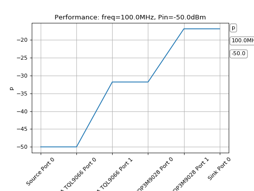
Here we see a simple plot. a so called sim.plot_chain(). “chained” because we see all the components in a signal chain, device after device. We see on the right side also some text information:

• p
• 100.00MHz
• -50.0dBm

the p is the current viewed variable, the middle is the current active frequency and the last one the current input power level. On some plots these items are clickable and will change when clicked or the mouseweel is used.

We will see more infos in a second.

Plotting

plot_chain

As we already saw, one of the plotting commands is called plot_chain. With this plot we see all the data-chain at a specific input frequency and at a specific power. This is a good view to analyse a system by scrolling through all the states and observe the hole component chain.

simResult.plot_chain(param=None, freq=None, power=None, keys=None)

plots a window with responsive fields which can be switched between (click or mousewheel)

plot_chain plots all data from the start to the end, by all ports between

we can select which ports to show, be defining the keys

when param, freq or power is not defined, all parameters will be shown

Parameters:

• param (str or list of str, optional) – a single parameter or a list of parameters which shall be plotted
• freq (float or list of floats, optional) – a single frequency or a list of frequencies which shall be plotted
• power (float or list of floats, optional) – a single power value or a list of power values which shall be plotted
• keys (str or list of str, optional) – a single device port or a list of device ports. only these values are extracted.

Notes

return handler must remain, otherwise the plot will not be responsive anymore

Returns:handler Return type:callback handlers

plot_total

In contrast to plot_chain we have the plot_total function. With this we see all the values at the end of the chain. The conclusion in some kind. We see a hole input power level sweep at a give frequency or a frequency sweep at a given input power.

With this kind of plot we can easily see the performance over the hole input range for a system.

simResult.plot_total(param=None, freq=None, power=None)

plots a window with responsive fields which can be switched between (click or mousewheel)

plot_total plots all “and” data in respect to frequency or power

we can select which ports to show, be defining the keys

when param, freq or power are not defined, all parameters will be shown

Parameters:

• param (str or list of str, optional) – a single parameter or a list of parameters which shall be plotted
• freq (float or list of floats, optional) – a single frequency or a list of frequencies which shall be plotted
• power (float or list of floats, optional) – a single power value or a list of power values which shall be plotted

Notes

return handler must remain, otherwise the plot will not be responsive anymore

Returns:handler Return type:callback handlers

plot_total_simple

Whereas the plot_total is an interactive window with clickable buttons, this plot_total_simple is static, more simplistic but gives the possibility to compare two different systems with each other.

For many RF application this plot together with the values ‘SNR’ and ‘SFDR’ resp. ‘Dynamic’ is a very informative plot to see where we loose SNR or Dynamic and vice versa where we got a sweetspot for both parameters.

simResult.plot_total_simple(param, freq=None, power=None, axis=None)

plots a window with the defined parameter

plot_total_simple is a simpler variant of the other plots

it is not a responvice view, but it is easy to show different parameters at once

Parameters:

• param (str or list of str) – a single parameter or a list of parameters which shall be plotted
• freq (float or list of floats, optional) – a single frequency or a list of frequencies which shall be plotted
• power (float or list of floats, optional) – a single power value or a list of power values which shall be plotted
• axis (axis object, optional) – currently not in use

Notes

return handler must remain, otherwise the plot will not be responsive anymore

Examples

>>> t = sim1.plot_total_simple(['SFDR', 'SNR', 'DYN'], freq=430e6)
>>> plt.show()

Returns:handler Return type:callback handlers

plot_surface

The plot_surface is used as a hole view to see the system at all input frequencies versus all input power levels at the same time.

simResult.plot_surface(param=None, freq=None, power=None, keys=None)

plots a window with responsive fields which can be switched between (click or mousewheel)

plot_surface plots a surface plot with all data in respect to al ports and power or frequency

we can select which ports to show, be defining the keys

when param, freq or power are not defined, all parameters will be shown

Parameters:

• param (str or list of str, optional) – a single parameter or a list of parameters which shall be plotted
• freq (float or list of floats, optional) – a single frequency or a list of frequencies which shall be plotted
• power (float or list of floats, optional) – a single power value or a list of power values which shall be plotted
• keys (str or list of str, optional) – a single device port or a list of device ports. only these values are extracted.

Notes

return handler must remain, otherwise the plot will not be responsive anymore

Returns:handler Return type:callback handlers

setNoiseBandwidth

We can adjust the noise-bandwidth of our system to adapt to our simulation needs. The script calculates internally in 1Hz resolution but shall be adjusted with this function.

simResult.setNoiseBandwidth(B)

set the noisebandwidth

changes the following parameters

• n : noise power
• SNR : signal to noise ratio
• DYN : dynamic

extract measurement data

extractValues

simResult.extractValues(param, freq, power, keys=None)

convencience function to access the data in a structured way

Parameters:

• param (str or list of str) – a single parameter or a list of parameters which shall be extracted
• freq (float or list of floats) – a single frequency or a list of frequencies which shall be extracted
• power (float or list of floats) – a single power value or a list of power values which shall be extracted
• keys (str or list of str, optional) – a single device port or a list of device ports. only these values are extracted.

Returns:

params – a tuple with all ports and the corresponding data

Return type:

(ports, data)

extractLastValues

simResult.extractLastValues(key, freq=None, power=None)

convencience function to access the data at the last device port.

an easy way to export all “end” values to compare systems with each other

Parameters:

• key (str) – a single device port or a list of device ports. only these values are extracted.
• freq (float, optional) – a single frequency or a list of frequencies which shall be extracted
• power (float, optional) – a single power value or a list of power values which shall be extracted

Returns:

params – data

Return type:

pandas.DataFrame