Introduction
This tool is used in three phases.
- First we define a circuit containing multiple devices.we connect those and maybe define some callback functions.
- In the second phase we simulate the circuit, define plots of interest.
- And in the third phase we optimize the circuit.
A simple example
First we define a simple circuit
We use two amplifiers in series
A Low Noise Amp and a Driver
 1import rf_linkbudget as rf
 2import matplotlib.pyplot as plt
 3import numpy as np
 4
 5cr = rf.Circuit('SimpleEx')
 6
 7lna = rf.Amplifier("LNA TQL9066",
 8                   Gain=[(0, 18.2)],
 9                   NF=0.7,
10                   OP1dB=21.5,
11                   OIP3=40)
12
13drv = rf.Amplifier("Driver TQP3M9028",
14                   Gain=[(0, 14.9)],
15                   NF=1.7,
16                   OP1dB=21.4,
17                   OIP3=40)
18
19src = rf.Source("Source")
20sink = rf.Sink("Sink")
Now we have to define connections between the devices
1src['out'] >> lna['in']
2lna['out'] >> drv['in']
3drv['out'] >> sink['in']
that we can simulate the circuit correctly, we have to define where the signal is applied to.
A Port as example.
We do this by using a callback function.
First we define it with an inline function, then connect this function to the Port by using the memberfunction called regCallback.
1# create callback function
2def cb_src(self, f, p):
3    return {'f': f, 'p': p, 'Tn': rf.RFMath.T0}
4
5
6src['out'].regCallback(cb_src)  # connect callback to Port
after defining all the callbacks we can finalize the circuit
1cr.finalise()
and simulate the circuit
1sim = cr.simulate(network=cr.net,
2                  start=cr['Source'],
3                  end=cr['Sink'],
4                  freq=[100e6],
5                  power=np.arange(-50, -10, 1.0))
6
7h = sim.plot_chain(['p'])
8
9plt.show()
We see that we have to define a start port and an end port.
In this case its intelligent enough to choose the cr[‘Source’][‘out’] port and the cr[‘Sink’][‘in’] port.
Also we have to define the frequency and input power range of the simulation
(Source code, png, hires.png, pdf)
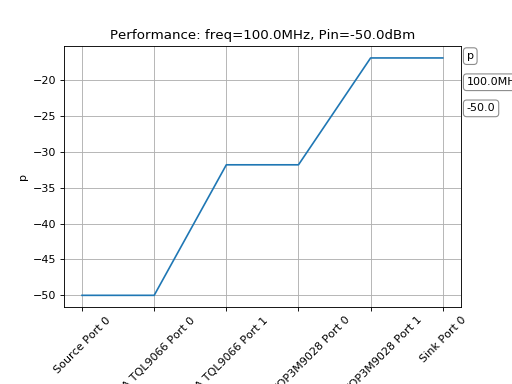
And here we see our output!
In this case we see the signal power p from the source to the sink.
We can also show other parameters like noisefigure, signal-to-noise ratio, spurious-free-dynamic-range and others.
 1import rf_linkbudget as rf
 2import matplotlib.pyplot as plt
 3import numpy as np
 4
 5cr = rf.Circuit('SimpleEx')
 6
 7lna = rf.Amplifier("LNA TQL9066",
 8                   Gain=[(0, 18.2)],
 9                   NF=0.7,
10                   OP1dB=21.5,
11                   OIP3=40)
12
13drv = rf.Amplifier("Driver TQP3M9028",
14                   Gain=[(0, 14.9)],
15                   NF=1.7,
16                   OP1dB=21.4,
17                   OIP3=40)
18
19src = rf.Source("Source")
20sink = rf.Sink("Sink")
21
22
23src['out'] >> lna['in']
24lna['out'] >> drv['in']
25drv['out'] >> sink['in']
26
27
28# create callback function
29def cb_src(self, f, p):
30    return {'f': f, 'p': p, 'Tn': rf.RFMath.T0}
31
32
33src['out'].regCallback(cb_src)  # connect callback to Port
34
35cr.finalise()
36
37
38sim = cr.simulate(network=cr.net,
39                  start=cr['Source'],
40                  end=cr['Sink'],
41                  freq=[100e6],
42                  power=np.arange(-50, -10, 1.0))
43
44h = sim.plot_chain(['p'])
45
46plt.show()