Circuit and Devices
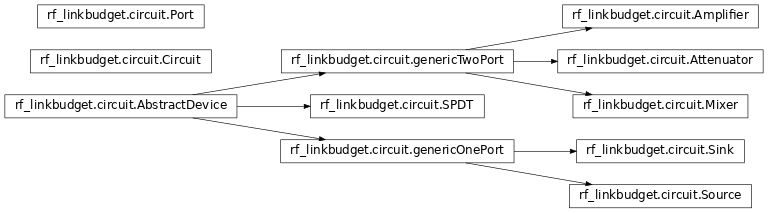
Class diagram
Circuit
The first step in every rf-linkbudget calculation is the creation of the circuit object
1import rf_linkbudget as rf
2cr = rf.Circuit("name of the circuit")
after that we have to create devices which are automatically added to the currently active circuit.
1lna = rf.Amplifier("LNA TQL9066",
2               Gain=[(0, 18.2)],
3               NF=0.7,
4               OP1dB=21.5,
5               OIP3=40)
We can access the amplifier in this example with the circuit object. This is just syntax sugar, but will be usefull when we want to configure plots
1print(cr["LNA TQL9066"])
2>>> <rf_linkbudget.circuit.Amplifier object at 0x7f1466e2b400>
As in the example we populate our circuit and define connections and register callback functions.
But when we’re done with that we want to finalise the circuit.
1cr.finalise()
This function makes some checks and creates a network object. A network of ports. We will see more in the next chapter about this. Lets just say for the moment, that we can model our circuit as a network of input and output ports which have a beginning and an end.
And after we finalised our circuit we want to simulate our results
1sim = cr.simulate(network=cr.net,
2                  start=cr['Source'],
3                  end=cr['Sink'],
4                  freq=[100e6],
5                  power=np.arange(-50, -10, 1.0))
We have to deliver our circuit as a network object, a starting port, an ending port a list of frequency points and a list of input power levels. Here we see the usefullness of the syntax sugar for referencing our devices by the circuit object.
The simulation makes a two dimensional matrix with frequency and power rows resp. columns. For every entry in this matrix there will be a full set of values calculated. like signal-to-noise ration, spurious-free-dynamic-range, but also concatenated Intermodulation point IP3 and compression point P1dB. But there will be an own chapter just for the calculations.
Lets just say for the moment, that the return object is from class simResult and does the hard-work…
Port
Every device we will use has at least one Port. Imagine the port as a model port from network theory. An amplifier will have two ports, an in and an out port. A source only has one port and 3dB hybrid will have 3 ports.
We can access the ports of a component by the number or for some devices which are non-reciproke with a string ‘in’ or ‘out’
 1lna = rf.Amplifier("LNA TQL9066",
 2               Gain=[(0, 18.2)],
 3               NF=0.7,
 4               OP1dB=21.5,
 5               OIP3=40)
 6
 7 print(lna['in'])
 8 >>> LNA TQL9066 Port 0
 9 print(lna['in'] == lna[0])
10 >>> True
11 print(lna['in'] == lna[1])
12 >>> False
13 print(lna['out'] == lna[1])
14 >>> True
As seen in the example we register a callback functions to a port. You probably assumed that the register callback function would be registered to the device object, but I decided to do it differently. As described before a circuit is a network of ports not a network of objects. This way around the calculations are more generalized.
Every port could be the start-or the end-port of a simulation. The network abstracts the point between ports as graphes and for every simulation an algorithm searches for the nearest distance between two ports and returns a directed graph from the start to the end port.
By defining the callback function to a port, we could also simulate the isolation of an amplifier in a generalized way and we would have to push our stimuli on the output port of this amplifier.
Callback Functions
We have to types of callback functions :
<port>.regCallback
<port>.regCallback_preIteration
The first regCallback is used to generate stimuli for a simulation. We can also use it to define the values of a step attenuator depending on the input power level
 1# create callback function
 2def cb_att1(self, f, p):
 3    tb = {-21: 2, -20: 3, -19: 4, -18: 5, -17: 6, -16: 7, -15: 8, -14: 9, -13: 10, -12: 11, -11: 12, -10: 13, }
 4    if(p in tb):
 5        self.setAttenuation(tb[p])
 6    else:
 7        self.setAttenuation(1.6)
 8    return {}
 9
10att1['in'].regCallback(cb_att1)
this way the attenuator can be regulated for the simulation. The regCallback gets called every frequency and power level the simulation was specified for. The Callback gets called just before calulating the input / output values of a device
And the second callback regCallback_preIteration is used to define settings for each iteration before calculating the individual device parameters. With this callback we can define system settings like if a mixer is an up- or downconverter, the mixer frequency and the noisefigure of the device depending on the LO frequency or power level.
We can refence inside the callback function to a temporary variable called Circuit.currentSimParams. Inside this variable all currently set Simulation Parameters are availlable.
1# create callback function
2def cb_att1(self, f, p):
3    ...
4    freq = Circuit.currentSimParams['freq']
5    start_node = Circuit.currentSimParams['start']
6    ...
We can use this feature to simulate more complex control schemes.
Devices
AbstractDevice
The AbstractDevice class is an Abstract Class. Other “real” devices will inherit this class.
It defines that every device has a name and at least one port. It calculates the internal port network. It also implements the behaviour that you can access the port by a key.
It defines an abstract function calcCurrentEdge which gets called by the Circuit class to calculate the output values. Every device has to implement this function by its own. And in this function only the “non-dependend” values are calculated.
It defines another function called calcAdditionalParameters which calculates all the other values based on the “non-dependend” values.
genericOnePort
The genericOnePort is an Abstract class itself, but also inherits AbstractDevice. It defines that device which inherit this class will exactly have one port and can be called by ‘in’, ‘out’ or ‘0’
genericTwoPort
The genericTwoPort is an Abstract class itself, but also inherits AbstractDevice. It defines that device which inherit this class will exactly have two ports where the input is called ‘in’ or ‘0’ and the output is ‘out’ or ‘1’ This class also implements the possibility to use a S2P file to import the device data directly. But be aware this script only extracts the S21 values.
- classmethod genericTwoPort.fromSParamFile(name, filename, Tn, P1, IP3, patchString='S12DB')[source]
- classmethod to create a two port device from a Touchstone S2P fileonly S21 is regarded
- Parameters:
name (str) – device name
filename (str) – S2P filename
Tn (list of [Tn @ Port 1, Tn @ Port 2]) – noisetemperature of object, represented at the “target” port [°K]
P1 (list of [P1 @ Port 1, P1 @ Port 2]) – Signal Compression Point of object, represented at the “target” port in [dB]
IP3 (list of [P3 @ Port 1, P3 @ Port 2]) – Signal Intermodulation Point 3 of object, represented at the “target” port in [dB]
patchString (str) – default ‘S12DB’
- Returns:
cls – object
- Return type:
genericTwoPort
The parameter patchString is a little bit odd. The author of the scikit-rf project which implements the touchstone importer actually only knows the generic n-port touchstone file format. The S2P touchstone format does arange the columns differently, thats why we need for extracting the S21 data of a S2P file the column “S12” which is at the same position for a n-port touchstone format as for the S21 values in an S2P touchstone file
Source
The Source is a one port device. It has an ‘out’ port and a name. Usually we use it as a starting point for our simulation
1src = rf.Source("Source")
2...
3
4src['out'] >> ...
Sink
The Sink is a one port device. It has an ‘in’ port and a name. Usually we use it as an ending point for our simulation
1sink = rf.Sink("Sink")
2...
3
4... >> sink['in']
Amplifier
The amplifier is a two port device. We can define it as following:
1lna = rf.Amplifier("LNA TQL9066",
2                   Gain=[(0, 18.2), (100, 18.0), (200, 17.8)],
3                   NF=0.7,
4                   OP1dB=21.5,
5                   OIP3=40)
We have to define at least a name, Gain, Noisefigure, OP1dB and OIP3 level. For the Gain we can also use a S2P file to import the data
1lna = rf.Amplifier.fromSParamFile("LNA TQL9066",
2                                  'data/TQL9066.s2p',
3                                  NF=0.7,
4                                  OP1dB=21.5,
5                                  OIP3=40)
The S2P importer only uses the S21 : Gain Information. (No embedded Noisefigure)
We can define the gain as a list of a tuple of frequency and gain.
Attenuator
An attenuator is also a classical two port device. It can be static or variable, defined by a range.
1att_fix = rf.Attenuator("Att Fix1",
2                      Att=[1.5])
First we see here the fixed attenuator case.
1dsa = rf.Attenuator("AFE79xx DSA",
2                     Att=np.arange(1.0, 29, 1.0))
And here a version with a defined range. We can now use a callback to parameterise.
 1dsa = rf.Attenuator("AFE79xx DSA",
 2                     Att=np.arange(1.0, 29, 1.0))
 3...
 4
 5# create callback function
 6def cb_dsa(self, f, p):
 7
 8  if(p > -20):
 9     self.setAttenuation(0.0)
10  else:
11     self.setAttenuation(15.6)
12  return {}
13
14  dsa['in'].regCallback(cb_dsa)
As we see in this example, we set the attenuator to 15.6dB for all input powers p below or equal -20dBm and set it to zero above it. The function setAttenuation will set it to the nearest attenuation value defined in the constructor. In this case the zero value will get set to effectively 1.0dB and the 15.6dB will be rounded up to 16.0dB.
Filter
An filter is a classical two port device. It has a frequency response
1filter = rf.Filter("Filter 1",
2                      Att=[(100, 1.5),(200, 4.5),(300, 55)])
As we see, we can define the frequency response like the frequency response of an Amplifier.
SPDT
1sw1 = rf.SPDT("SW 1",
2                Att=0.3)
3...
4
5sw1['S-1'] >> att1['in']
6att1['out'] >> sw2['S-1']
7sw1['S-2'] >> sw2['S-2']
Has ports ‘S’, ‘S-1’, ‘S-2’
 1# create callback function
 2  def cb_sw1(self, f, p):
 3      if(p < -21):
 4          self.setDirection('S-2')
 5      else:
 6          self.setDirection('S-1')
 7      return {}
 8
 9  sw1['S'].regCallback(cb_sw1)
10  sw2['S'].regCallback(cb_sw1)
We can also specify the isolation in case of a malconfigured switch
1sw1 = rf.SPDT("SW 1",
2                Att=0.3, Iso=60)
3...
Mixer
1mix = rf.Mixer("MIY SYM-18+",
2                   Gain=[(0, -8.61), (100, -8.41), (200, -8.64)],
3                   OP1dB=14,
4                   OIP3=30)
The single-sideband noisefigure is equal to the insertion loss of the mixer. We will add the sideband-noise in the callback function
As we will see there is the therm : (10**(Att/10) * rf.RFMath.T0 - rf.RFMath.T0) which adds the sideband noise term. In this case the sideband-noise is suppressed down to the noisefloor and will add 3dB noisefigure. We can also simulate the influence of higher sideband noise the same way.
1# create callback function
2def cbI_mix(self, data, f, p):
3    # upconverter with flo = 100MHz
4    data.update({'f': f + 100e6})
5    # add 3dB noise Figure due to sideband noise
6    data.update({'Tn': data['Tn'] + (10**(3/10) * rf.RFMath.T0 - rf.RFMath.T0)})
7    return data
8
9mix['in'].regCallback_preIteration(cbI_mix)  # connect callback to Port
There are two important things to notice here:
The callback function we use is calleg regCallback_preIteration() this callback will be called each iteration for each component
The callback function must be attached at the ‘in’ port
In the callback function we manipulate the data[‘f’] parameter. We can simulate the influence of the frequency conversion with it. Usually the Gain and Noise Values are referenced by data[‘f’]. But in the case, where we mix to a fixed output frequency this is leads to a wrong output values. (because we would use always the same gain / noise values because the output frequency, where we reference on is always the same) We can define in the callback function the following code to define an own reference frequency:
1# create callback function
2def cbI_mix(self, data, f, p):
3    ...
4    data.update({'f_ref': f + 100e6})
5    ...
6    return data
This way the code will use ‘f_ref’ as refence for the calculations.
Duplexer
TODO